Logistic regression classification models
The notebook used to develop the logistic regression models iterpreted below can be found here.
Summary
Following the creation of our inital baseline model, as described and interpreted on this page, where we used logistic regression with only lat and lon as our predictors, we then expanded our model to our entire feature-set for predictiing crime-type classes for each crime record. This page describes these additional logistic regression classifier modeling efforts and provide an interpretation of the results. For a full predictor-by-predictor listing of the predictors used in the models on this page, along with a brief description of each predictor, please see this section of our “Models” page. Please note that, for all models on this page in which we have used our entire feature set, all non-binary predictor values have been scaled using standardization with the training set used as our reference set for calculating the means and standard deviations with which to scale both the training and test values.
Below we have also chosen to test a comparable set of logistic regression models, wherein we seek to predict a smaller subset of crime-type classes in an attempt to overcome some of our class imbalance challenges and to better understand the effect of reduced class categories on our model. A detailed listing of the full set of crime-type response classes can be found here, and a description of the comparative secondary set of reduced classes can be found here.
Contents
Contained on this page are results and interpretations for the following models:
- Model 1: Logistic regression classifier without regularization
- Model 2: Logistic regression with cross-validated l1 regularization
- Model 3: Baseline logistic regression with subsetted classes
- Model 4: Logistic regression with subset classes and CV l1 regularization
Model 1: Logistic regression classifier without regularization
Model 1 parameters
For the initial model that we investigate on this page, we train a logistic regression classifier without regularization, as a point of comparison with our initial baseline model. Once again, we trained two versions of our model, one without any class weighting applied to the model, and a second with “balanced” class weightings applied.
The parameters of the two scikit-learn LogisticRegression model objects fitted for our baseline model are:
MODEL 1.a.: Without balanced class weights
LogisticRegression(C=100000, class_weight=None, dual=False,
                   fit_intercept=True, intercept_scaling=1,
                   l1_ratio=None, max_iter=1000,
                   multi_class='multinomial', n_jobs=None,
                   penalty='l2', random_state=20, solver='lbfgs',
                   tol=0.0001, verbose=0, warm_start=False)
MODEL 1.b.: With balanced class weights
LogisticRegression(C=100000, class_weight=None, dual=False,
                   fit_intercept=True, intercept_scaling=1,
                   l1_ratio=None, max_iter=1000,
                   multi_class='multinomial', n_jobs=None,
                   penalty='l2', random_state=20, solver='lbfgs',
                   tol=0.0001, verbose=0, warm_start=False)
Model 1 accuracy and AUC
Ultimately, these models resulted in the following training accuracies and average AUCs. As we can see the Model 1.a. generated without using balanced class weights acheived only a TEST accuracy of 0.2965, a 2 point improvement over the 0.2733 achieved with our baseline model. What this indicates to us is that, with our entire predictor set (versus using just lat and lon in our baseline model), the logistic regression classifier can more easily separate out crime-type classes in its prediction. Rather than using geo-spatial coodinates, two dimensions on which our crime-type classes are heavily mixed and difficult to separate in a linear manner, we now have a large set of additional dimensions on which to evaluate each crime record. This appears to have improved the predictive strength of our model.
Another characteristic to note is that our TEST AUC has been even more strongly improved than our accuracy. Whereas in our baseline model our unweighted TEST AUC was 0.537, with all of our predictors added, our Model 1.a. achieves a TEST AUC of 0.617, a clear improvement.
Most notable in the results below are those that we achieve in Model 1.b, where we applied “balanced” class weightings while fitting our model. As can be seen below, our Model 1.b. prediction accuracy was 0.2131, much improved over the 0.1331 acheived in our balanced baseline model. Once again here, as we saw with our baseline models, the TEST AUC is once again comparable between our balanced and unbalanced models, indicating that the AUC metric suffers much less so than accuracy when balancing our our class weights.
MODEL 1.a.: Without balanced class weights
This model resulted in the following accuracy:

Training	0.2965
Test		0.2977

The model AUC is:

		weighted    unweighted
Training	0.6264		0.6221
Test		0.6235		0.6171
MODEL 1.b.: With balanced class weights
This model resulted in the following accuracy:

Training	0.2131
Test		0.2131

The model AUC is:

		weighted	unweighted
Training	0.6246		0.6205
Test		0.6215		0.6152
Model 1 predictions
By viewing the confusion matrices generated by each version of the Model 1, we can see that, unlike our baseline model without class weighting, with our full predictor-set our new Model 1.a. generates predictions for almost all of our crime-type response classes. The only exception, visible in the first table below, is crime-type class 5 (robbery) which also happens to represent the crime-type class with the lowest proportion of true observations among all of our crime-type classes as was shown in the response variable summary table on our “Models” page. And, as we’d expect Model 1.b. with balanced class weighting generates predictions for all of our crime-type response classes, including class 5. These results, particularly for Model 1.a., indicate to us that our full set of predictors does a good job at beginning to separate response classes for the model, even with the severe class imbalances in our training set.
MODEL 1.a.: Without balanced class weights
The resulting confusion matrix:

TEST
Actual        0     1     2     3     4    5     6     7     8  Total
Predicted
0             0     0     0     1     0    0     0     1     1      3
1             0     0     0     0     1    0     0     1     0      2
2            62    70   459   105   190   40   312   131   239   1608
3             1     0     0     3     0    0     4     0     0      8
4           391   434   820   651  2531  258  1816  1163  1833   9897
5             0     0     0     0     0    0     0     0     0      0
6           984   816  1844  1515  2090  477  6091  1863  2773  18453
7             0     0     0     1     1    1     5     5     0     13
8           142    96   148   121   379   80   411   263   464   2104
Total      1580  1416  3271  2397  5192  856  8639  3427  5310  32088
MODEL 1.b.: With balanced class weights
The resulting confusion matrix:

TEST
Actual        0     1     2     3     4    5     6     7     8  Total
Predicted
0           375   130   349   262   494  107   982   368   721   3788
1           162   277   276   351   543   66   920   431   461   3487
2           241   248  1271   429   802  182  1558   585   898   6214
3            73    66   156   189   232   38   458   179   233   1624
4           337   345   685   523  2191  218  1653   982  1591   8525
5           100   124   180   156   347  103   521   257   454   2242
6           202   127   236   388   295   83  2119   358   578   4386
7            73    79    91    75   216   44   319   207   269   1373
8            17    20    27    24    72   15   109    60   105    449
Total      1580  1416  3271  2397  5192  856  8639  3427  5310  32088
Model 1 receiver operator characteristic (ROC) curves by model and class
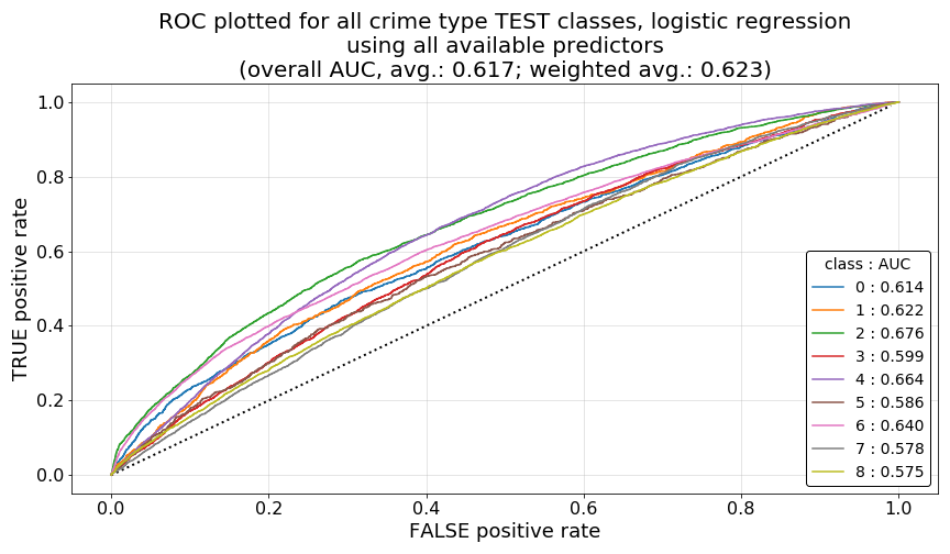
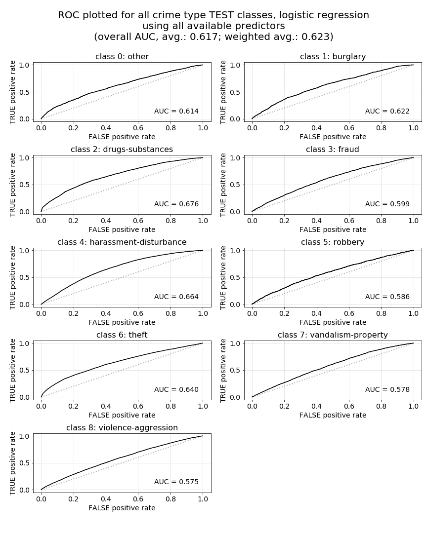
As was discussed in our analysis of our baseline model’s ROC curves, we are hoping to see curves for each class that rise very steeply toward a true positive rate (TPR) of 1.0 at very low values for the corresponding false positive rates (FPR), idealing forming a very high, far left, sharp elbow in each curve. While our Model 1.a. ROC curves do not exemplify those visual characteristic, they are visually far improved over the curves we saw in our baseline model as per the reasons described there.
Shown in the plots below, we can see that our Model 1.a. ROC curves have all begun to bow upward and away from the dashed reference line at which AUC would be equal to 0.50. While some crime-type class ROC curves appear to be more favorable than others, drugs-substances, harassment-disturbance, and theft stand out as exhibiting the best properties. Overall, the class-by-class shapes of these curves support what we would expect to see with the improved 0.62 average TEST AUC, which improved over the 0.54 generated by our baseline model.
Model 2: Logistic regression classifier with cross-validated lasso (l1) regularization
Now, to better understand which predictors are more important to each crime-type class and to see if we can gain any predictive benefits via regularization, we generate a cross-validated model using lasso-like (l1) regularization. Doing so will shrink our coefficients, and once plotted, will illustrate which coefficients were found insignificant for particular classes.
Model 2 parameters
To improve our measurement of each predictor’s effect on our crime-type type classes, we decided to balance our class weights in this model. Additionally, because we will likely find the true positive rate versus false positive rate tradeoff for particular classes more important than our overall model accuracy, we have also decided to use roc_auc_ovr as our cross-validation scoring metric, as opposed to the default metric accuracy. For our values C controlling our regularization parameter, we left scikit-learn’s default parameters in place. Below are the final parameters applied to our fitted LogisticRegressionCV model.
MODEL 2: CV lasso regularized, with balanced class weights
LogisticRegressionCV(Cs=10, class_weight='balanced',
                     cv=None, dual=False, fit_intercept=True, intercept_scaling=1.0, l1_ratios=None,
                     max_iter=1000, multi_class='multinomial',
                     n_jobs=None, penalty='l1', random_state=20,
                     refit=True, scoring='roc_auc_ovr',
                     solver='saga', tol=0.0001, verbose=0)
Model 2 accuracy and AUC
Similar to what we saw with our un-regularized Model 1.a. with balanced class weights, this model too achieves a TEST accuracy of only 0.2133 and an unweighted average AUC of 0.6152, indicating that we gain no significant predictive enhancements by regularizing our coefficients.
MODEL 2: CV lasso regularized, with balanced class weights
This model resulted in the following accuracy:

Training	0.2133
Test		0.2133

The model AUC is:

		weighted	unweighted
Training	0.6246		0.6205
Test		0.6215		0.6152
Model 2 predictions
As we’d expect, with our balanced class weights, this model distributes its TEST predictions across all crime-type classes, and it appears that class 4 (harassment-disturbance), class 2 (drugs-substances), and class 6 (theft) achieve the highes true-positive prediction rates (TPR). These three classes are also ones representing a particularly high proportion of all observations in our training and test sets.
MODEL 2: CV lasso regularized, with balanced class weights
The resulting confusion matrix:

TEST
Actual        0     1     2     3     4    5     6     7     8  Total
Predicted
0           378   129   351   261   498  108   982   367   726   3800
1           160   280   275   354   542   66   920   432   465   3494
2           240   248  1269   433   803  184  1558   590   896   6221
3            70    65   150   182   226   39   448   176   229   1585
4           340   344   693   527  2201  220  1661   987  1602   8575
5            99   128   179   154   344  100   515   258   446   2223
6           205   128   235   388   294   80  2129   359   578   4396
7            71    75    94    74   214   44   314   201   264   1351
8            17    19    25    24    70   15   112    57   104    443
Total      1580  1416  3271  2397  5192  856  8639  3427  5310  32088

The classification metrics derived from the confusion matrix are:

TEST
         TP    FP    FN     TN    TPR    FNR    FPR    TNR
class
0       378  3422  1202  27086  0.239  0.761  0.112  0.888
1       280  3214  1136  27458  0.198  0.802  0.105  0.895
2      1269  4952  2002  23865  0.388  0.612  0.172  0.828
3       182  1403  2215  28288  0.076  0.924  0.047  0.953
4      2201  6374  2991  20522  0.424  0.576  0.237  0.763
5       100  2123   756  29109  0.117  0.883  0.068  0.932
6      2129  2267  6510  21182  0.246  0.754  0.097  0.903
7       201  1150  3226  27511  0.059  0.941  0.040  0.960
8       104   339  5206  26439  0.020  0.980  0.013  0.987
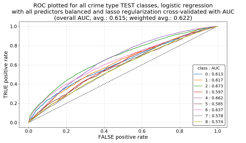
Model 2 receiver operator characteristic (ROC) curves by class
Then, when we inspect our ROC curves for each of the classes, we can again see curves similar to what was shown above in Model 1, as we’d expect given Model 2’s similar overall average AUC score.
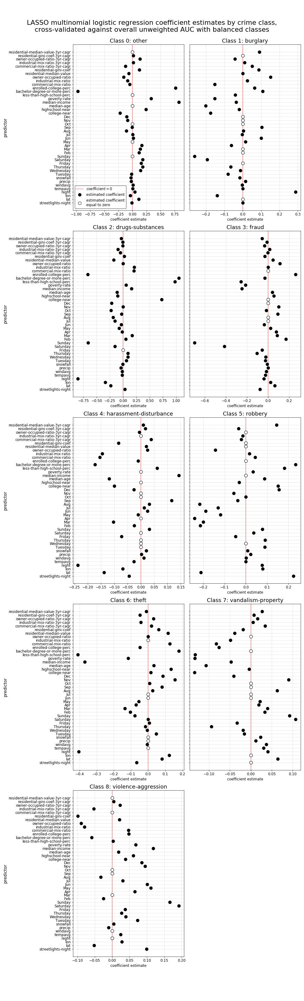
Model 2 lasso regularized coefficients
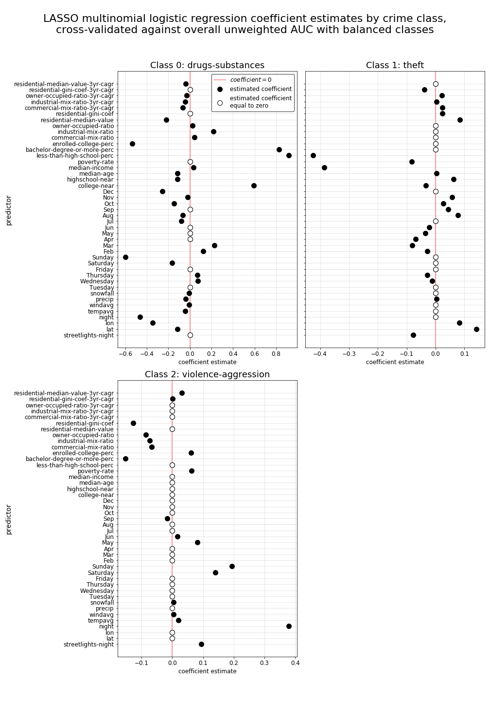
Finally, with lasso regularized shrinkage applied to our coefficients, we can now plot each coefficient estimate for every individual crime-type class (as is shown below) to identify the relationships of specific predictors to the predicted propability of each crime-type occuring over all others, and we can also see which predictors are considered insignificant by the model for each class’s individual prediction (as is evidenced by a coefficient estimate of zero in the plots below). While there is a lot of information to take in while viewing the plots below, by looking at some of the predictors with the largest coefficients, we can begin to see some relationships surface that we may expect. For instance, weekend days (Saturday and Sunday) appear to have high predictive strength for violence-aggression type crimes, while the property-related inequality measure residential-gini-coef and the night indicator both appear to have strong positive relationships to burglary predictions. While overall accuracy of our model isn’t particularly high, the interpretability of these coefficient estimate results can at least give us a glimpse into the interactive relationships of each of these predictors among our crime-type classes, informing future modeling decisions and helping us to determine how we might reengineer some of our predictors to simplify our model and hopefully make it more accurate when we apply other types of classification methods.
Model 3: Baseline logistic regression with subsetted crime-type classes
As a comparative analysis and an attempt to overcome the imbalanced classes existing in our primary set of crime-type classes, we have chosen to also generate predictive models using a smaller subset of our classes as was described on our “Models” page. In doing so, we are also able to examine potential changes in predictive accuracy when the number of overall classes are reduced. For reference, this reduced subset of classes includes:
class       class-name
0           drugs-substances
1           theft
2           violence-aggression
Model 3 parameters
As a new baseline, we first generate a logistic regression model on our subsetted classes using just lat and lon as predictors as we did before with our larger class set. No class weights are applied in this model. The parameters set for this model are shown below.
MODEL 3: Subset classes, baseline, without weights
LogisticRegression(C=100000, class_weight=None, dual=False,
                   fit_intercept=True, intercept_scaling=1,
                   l1_ratio=None, max_iter=1000, multi_class='multinomial', n_jobs=None, penalty='l2', random_state=20,
                   solver='lbfgs', tol=0.0001, verbose=0, warm_start=False)
Model 3 accuracy and AUC
Immediately, with a TEST accuracy score of 0.478 we can see a large gain in the overall accuracy of our model as compared to our previous models (all below 0.30 accuracy). This is surprising, considering the poor performance we say in our original baseline model, which also used just lat and lon as predictors. However, something else that is noticeable is the lack of improvement in AUC performance with this model.
MODEL 3: Subset classes, baseline, without weights
This model resulted in the following accuracy:

Training	0.4785
Test		0.4779

The model AUC is:

		weighted	unweighted
Training	0.5760		0.5706
Test		0.5768		0.5709
Model 3 predictions
Below we can see, that without balanced class weights applied to our model, the remaining imbalances in our three crime-type classes, lead to a model that failed to predict a single occurance of class 0 (drugs-substances) crimes. But, by inspective the classification metrics table below, we can see a notable improvement in the true positive rate (TPR) for our class 2 (violence-aggression) predictions. In our prior models, the best that we achieved for this class was a TPR of 0.02.
MODEL 3: Subsetted classes, baseline, without weights
The resulting confusion matrix:

TEST
Actual        0     1     2  Total
Predicted
0             0     0     0      0
1          2719  7485  5012  15216
2           552  1154  1154   2860
Total      3271  8639  6166  18076

The classification metrics derived from the confusion matrix are:

TEST
         TP    FP    FN     TN    TPR    FNR    FPR    TNR
class
0         0     0  3271  14805  0.000  1.000  0.000  1.000
1      7485  7731  1154   1706  0.866  0.134  0.819  0.181
2      1154  1706  5012  10204  0.187  0.813  0.143  0.857
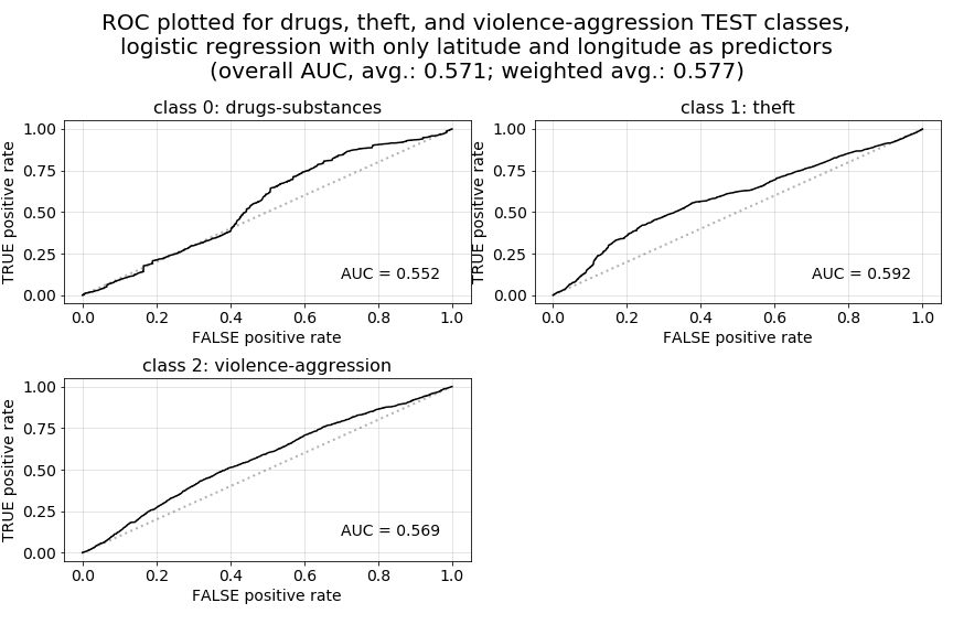
Model 3 receiver operator characteristic (ROC) curves by class
Finally, and somewhat disappointingly, we can see less than favorable results in our ROC curves, indicating that we have little opportunity for improving true positive rates without significance cost in terms of increase false positive rates by adjusting the thresholds of particular response classes.
Model 4: Logistic regression with subset classes and cross-validation lasso (l1) regularization
Model 4 parameters
Now, as a final comparative exercise, we will generate a logistic regression model on our subsetted crime-type class set using all predictors in our feature set. Once again we will apply cross-validated lasso regularization to our coefficients. And, similar to Model 2, we will also use roc_auc_ovr as our cross-validation scoring metric and we will once again balance our class weights to improve our measurement of each predictor’s effect on each class type. Below are the full set of parameters applied to this fitted LogisticRegressionCV model in scikit-learn.
MODEL 4: Subset classes, CV lasso regularization, balanced weights
LogisticRegressionCV(Cs=10, class_weight='balanced', cv=None,
                     dual=False, fit_intercept=True, intercept_scaling=1.0, l1_ratios=None, max_iter=1000, multi_class='multinomial', n_jobs=None, penalty='l1', random_state=20, refit=True,
                     scoring='roc_auc_ovr', solver='saga', tol=0.0001,
                     verbose=0)
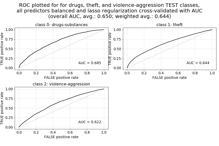
Model 4 accuracy and AUC
Here we can see that, while our test accuracy score dropped slightly below what we had achieved in our Model 3 baseline model (however still at a level well above what we had achieved in Model 1 and Model 2), we have now managed to regain a stronger overall AUC for our predictions. At 0.650 unweighted for our test predictions, this AUC also surpasses the best we had seen in our prior models.
MODEL 4: Subset classes, CV lasso regularization, balanced weights
This model resulted in the following accuracy:

Training	0.4599
Test		0.4510

The model AUC is:

		weighted	unweighted
Training	0.6498		0.6578
Test		0.6435		0.6500
Model 4 predictions
Looking at our resulting confusion matrix, we can see what we’d expect to occur when using balanced class weights in our model. We now have predictions distributed across all crime-type classes. We also have much higher true positive rates (TPRs) for class 0 and class 2 predictions (0.564 and 0.442 respectively), apparently at the cost of TPR accuracy for class 1 predictions, which would explain the overall drop in this model’s accuracy score.
The resulting confusion matrix:

TEST
Actual        0     1     2  Total
Predicted
0          1844  2555  2026   6425
1           578  3581  1413   5572
2           849  2503  2727   6079
Total      3271  8639  6166  18076

The classification metrics derived from the confusion matrix are:

TEST
         TP    FP    FN     TN    TPR    FNR    FPR    TNR
class
0      1844  4581  1427  10224  0.564  0.436  0.309  0.691
1      3581  1991  5058   7446  0.415  0.585  0.211  0.789
2      2727  3352  3439   8558  0.442  0.558  0.281  0.719
Model 4 receiver operator characteristic (ROC) curves by class
Now, as a point of comparison below, we provide both the ROC curve plots for our current Model 4 version (the first set of plots below), as well as a set of ROC curve plots for a prior iteration of Model 4 (the second set of plots) in which we used accuracy as our cross-validation scoring metric instead of roc_auc_ovr. Because we have chosen to priorities AUC over raw accuracy in our predictions, these two plots illustrate the very different outcomes we get in terms of AUC when accuracy is used for scoring and parameter selection during cross-validation. The first set of ROC curves illustrate far more favorable characteristics.

Model 4 lasso regularized coefficients
Finally, when looking at our lasso regularized coefficients for this version of the model, we can see that a far larger number of our coefficients estimates have been shrunk to zero. This would make sense, given that there are a much smaller number of crime-type classes for our model to differentiate between, leading to fewer predictors required for each class’s prediction.