Baseline model using logistic regression
The notebook used to develop this baseline model can be found here.
Summary
As an initial baseline model, against which we could compare the results of our subsequent models, we attempted to predict crime types using only latitude and longitude (lat and lon) as our predictors. To accomplish this, we ran a multinomial logistic model with no regularization. And we ran it both with and then without “balanced” class weightings for comparison. Given the heavy spatial mixing of crime-type classes as shown in our initial training data EDA we had very low expectations for the quality of predictions that might be generated using only geo-spatial coordinates as our predictors.
Model parameters
For comparison the parameters of the two scikit-learn LogisticRegression model objects fitted for our baseline model are:
MODEL 1: Without balanced class weights
LogisticRegression(C=100000, class_weight=None, dual=False,
                   fit_intercept=True, intercept_scaling=1,
                   l1_ratio=None, max_iter=1000,
                   multi_class='multinomial', n_jobs=None,
                   penalty='l2', random_state=20, solver='lbfgs',
                   tol=0.0001, verbose=0, warm_start=False)
MODEL 2: With balanced class weights
LogisticRegression(C=100000, class_weight=None, dual=False,
                   fit_intercept=True, intercept_scaling=1,
                   l1_ratio=None, max_iter=1000,
                   multi_class='multinomial', n_jobs=None,
                   penalty='l2', random_state=20, solver='lbfgs',
                   tol=0.0001, verbose=0, warm_start=False)
Model accuracy and AUC
Ultimately, these models resulted in the following training accuracies and average AUCs. As we can see the model generated without using balanced class weights acheived only a TEST accuracy of just 0.2733, which is not surprising given the expected difficulty of predicting crime types given our previous exploration of this data. However, what is interesting is the far lower TEST accuracy for the Model 2, generated using balanced class weights. Surprisingly, the AUC of Model 2 suffers very little as a result of balancing class weights, which leads us to further inspect the prediction results generated by each model in the next section below.
MODEL 1: Without balanced class weights
This model resulted in the following accuracy:

Training	0.2706
Test		0.2733

The model AUC is:

	        weighted	unweighted
Training	0.5519		0.5396
Test		0.5558		0.5370
MODEL 2: With balanced class weights
This model resulted in the following accuracy:

Training	0.1295
Test		0.1332

The model AUC is:

		    weighted	unweighted
Training	0.5487		0.5382
Test		0.5529		0.5395
Model predictions
By viewing the number of predictions generated by each version of the model, we can see that Model 2 generated a more balanced set of predictions, whereas Model 1 only predicted occurances of crime-type classes 4 (harassment-disturbance) and 6 (theft), two of the most heavily over-represented classes in our training set. Even with some many false negative predicted for all other classes in Model 1, because these two classes together represent 43% of our total true TEST observations, this would explain why were able to achieve the TEST accuracy score we did with that model. Likewise, because Model 2 predictions are distributed among all potential response classes, the heavy over-representation of crime-type classes 0 (other) and 4 in our results very negatively impacts overall accuracy on the test set.
MODEL 1: Without balanced class weights
The number of classes predicted by class are:

TRAINING
        count  proportion
class
4       15446    0.120341
6      112906    0.879659

TEST
       count  proportion
class
4       3939    0.122756
6      28149    0.877244
MODEL 2: With balanced class weights
The number of classes predicted by class are:

TRAINING
       count  proportion
class
0      53841    0.419479
1       6662    0.051904
2       1595    0.012427
3       2222    0.017312
4      52740    0.410901
5       3164    0.024651
6       3877    0.030206
7       1837    0.014312
8       2414    0.018808

TEST
       count  proportion
class
0      13476    0.419970
1       1624    0.050611
2        423    0.013182
3        527    0.016424
4      13313    0.414890
5        763    0.023778
6        964    0.030042
7        409    0.012746
8        589    0.018356
To further understand this effect, we can look at the confusion matrices and resulting classification metrics generated by the TEST results of each model as are shown below. Here again we can see the result of Model 2 predicting a larger number of response classes for the TEST set. For example, the true positive rate (TPR) shown for crime-type 6 in Model 1 is 0.905, but in Model 2 TPR for this same class drops to just 0.026. Because crime-type 6 is our most heavily represented class in our actual TEST data, this metric too supports the discrepancy in Model 1 versus Model 2 accuracy results that we have seen.
MODEL 1: Without balanced class weights
The resulting confusion matrix:

TEST
Actual        0     1     2     3     4    5     6     7     8  Total
Predicted
0             0     0     0     0     0    0     0     0     0      0
1             0     0     0     0     0    0     0     0     0      0
2             0     0     0     0     0    0     0     0     0      0
3             0     0     0     0     0    0     0     0     0      0
4           127   154   329   357   954  105   824   458   631   3939
5             0     0     0     0     0    0     0     0     0      0
6          1453  1262  2942  2040  4238  751  7815  2969  4679  28149
7             0     0     0     0     0    0     0     0     0      0
8             0     0     0     0     0    0     0     0     0      0
Total      1580  1416  3271  2397  5192  856  8639  3427  5310  32088

The classification metrics derived from the confusion matrix are:

TEST
         TP     FP    FN     TN    TPR    FNR    FPR    TNR
class
0         0      0  1580  30508  0.000  1.000  0.000  1.000
1         0      0  1416  30672  0.000  1.000  0.000  1.000
2         0      0  3271  28817  0.000  1.000  0.000  1.000
3         0      0  2397  29691  0.000  1.000  0.000  1.000
4       954   2985  4238  23911  0.184  0.816  0.111  0.889
5         0      0   856  31232  0.000  1.000  0.000  1.000
6      7815  20334   824   3115  0.905  0.095  0.867  0.133
7         0      0  3427  28661  0.000  1.000  0.000  1.000
8         0      0  5310  26778  0.000  1.000  0.000  1.000
MODEL 2: With balanced class weights
The resulting confusion matrix:

TEST
Actual        0     1     2     3     4    5     6     7     8  Total
Predicted
0           697   479  1532  1088  1207  394  4715  1245  2119  13476
1           102    85    97    98   353   50   383   173   283   1624
2            21    21    27    30    85    6   120    46    67    423
3            29    24    24    28    99   16   125    73   109    527
4           525   675  1246   974  3041  320  2690  1572  2270  13313
5            41    46   122    51   101   25   155    79   143    763
6           114    32   112    62   133   25   222   100   164    964
7            16    30    30    25    79    8    88    64    69    409
8            35    24    81    41    94   12   141    75    86    589
Total      1580  1416  3271  2397  5192  856  8639  3427  5310  32088

The classification metrics derived from the confusion matrix are:

TEST
         TP     FP    FN     TN    TPR    FNR    FPR    TNR
class
0       697  12779   883  17729  0.441  0.559  0.419  0.581
1        85   1539  1331  29133  0.060  0.940  0.050  0.950
2        27    396  3244  28421  0.008  0.992  0.014  0.986
3        28    499  2369  29192  0.012  0.988  0.017  0.983
4      3041  10272  2151  16624  0.586  0.414  0.382  0.618
5        25    738   831  30494  0.029  0.971  0.024  0.976
6       222    742  8417  22707  0.026  0.974  0.032  0.968
7        64    345  3363  28316  0.019  0.981  0.012  0.988
8        86    503  5224  26275  0.016  0.984  0.019  0.981
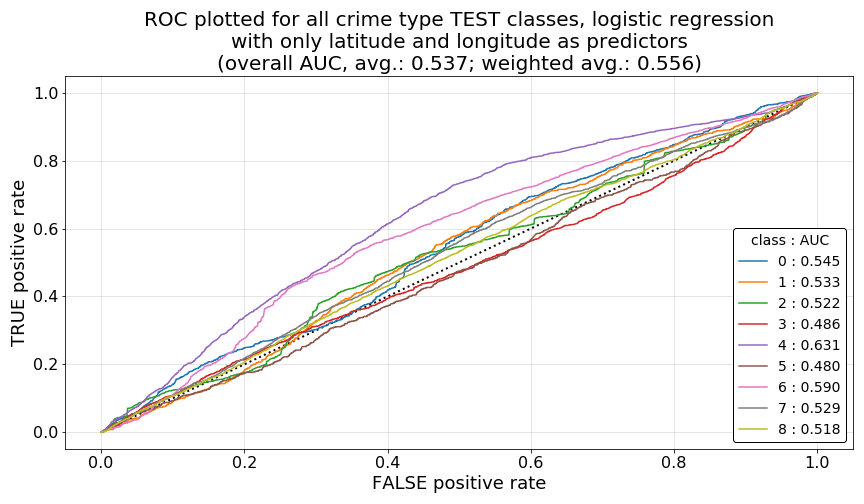
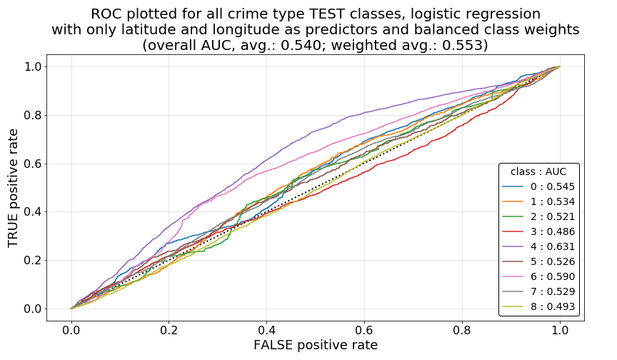
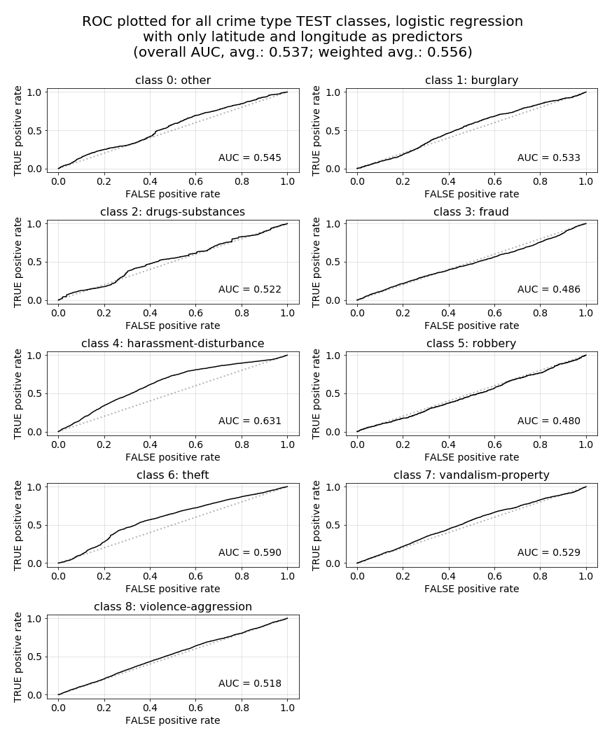
Receiver operator characteristic (ROC) curves by model and class
As a final set of items we will investigate to better understand these quality of our results and the differences that we are seeing between Model 1 and Model 2, we will now plot the ROC for each model and class, and report on the individual AUC values by class and model.
As we can see in the first two plots below, ROC curve plotted by class for each model shows very similar results among Model 1 and Model 2 (plotted in that order below), explaining the very similar average overall AUC for both models (note that this metric is also reported on the plots). However, what is evident in both of these models are the unfavorable overall ROC curve shapes for all classes, even the best performing class, crime-type class 4. What we would hope to see here are ROC curves rising very steeply toward a true positive rate (TPR) of 1.0 at very low values for the corresponding false positive rates (FPR), idealing forming a very high, far left, sharp elbow in each curve. Such a curve would indicate that, by modifying our classification probability thresholds for each class (or a particular class of interest, such as violence-aggression) there would be a very low trade-off in FPR to achieve higher TPRs for individual class predictions. A good illustrative example of this this relationship can be seen on the related Wikipedia article, most notably in the illustrative image located here.
However, what we see in our plots below are wavering ROC curves with very low rates of increase across each plot. Notably, some class ROC curves are even at or below the 0.5 AUC threshold, as is indicated by curved below the diagonal dashed black line plotted as a point of interest in each figure. This particular relationship to the AUC=0.5 reference line can be more easily seen in the third plot below, which breaks out ROC curves for each individual crime-type class for Model 1 as a visual example. Ideally, in future models, would like to see each of these curves pulled upward, toward the left, and away from that 0.5 AUC dashed line as far as possible, which would indicate more favorable opportunities for increasing TPR for particular crime-type classes of interest.
Conclusion and next steps
As expected from our initial EDA and data visualization efforts, due to the heavy spatial mixing of crime-type classes, we have achieved very low accuracy scores and far less than favorable AUC values and ROC curves with the two versions of our baseline model above. What’s also interesting is the sharp decrease in accuracy we achieve when balancing the class weights of our fitted model as discussed above. These are both challenges we will seek to address in our subsequent models.
To some degree, we expect that logistic regression will fail to adequately separate prediction classes due to the linear nature of the model, and that we will eventually find better results by using non-parametric methods such as k-Nearest Neighbors classifiers or Decision Tree-based classifiers, which can provide more flexible decision boundaries. However, after viewing these results, we were still very interested to see what additional predictive accuracy we could achieve and how different our AUC and ROC results might be once we add in a more complete predictor set. To view the results of our subsequent Logistic Regression classifier models in which we generated predictions using the entire set of predictors, please see the Logistic Regression Classifiers summary page. As you can see on that page, we were able to achieve some very interesting results, even with just logistic regression as our classifier.