The Decision Tree notebook can be found here.

After exploring the baseline model we examined several Decision Tree Classifier models. The Decision Tree model with tuning does a fair job with the data and reaches a max accuracy of approximately 0.35 with nine classes of crime.

Decision Tree Model

In an effort to create the most efficient decision tree model we first explored tree scores at various tree depths utilizing 5-fold cross validation.

The plot below shows that at a depth of 11 we have the highest mean CV score. The standard deviation at depth=11 is also not too wide. Depths 11-13 are very similar so any of those could potentially work and have been tested.

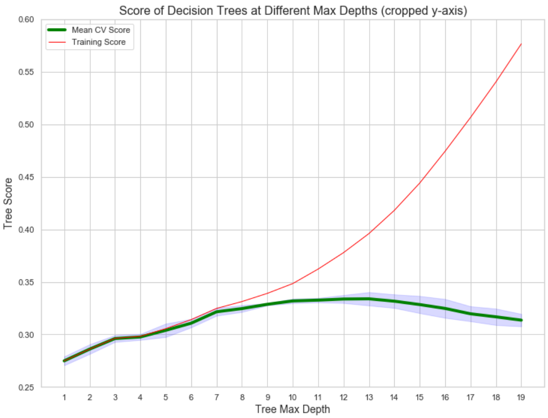
Given our optimal mean CV score we built our first model called “best_cv_tree” model with the max_depth parameter set to 11:

best_cv_tree = DecisionTreeClassifier(max_depth=11) 

best_cv_tree produced a training accuracy of 0.3622 and a test accuracy of 0.3358.

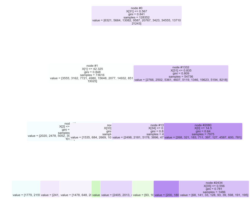
Top Predictors

Digging deeper into our initial tree model we sought to better understand our top predictors. The following image creates a tree diagram to visually illustrate the ranked importance of our top predictors.

tree_plot

The table below takes those same top predictors and produces a more user-friendly table with column names:

tree_top_predictors

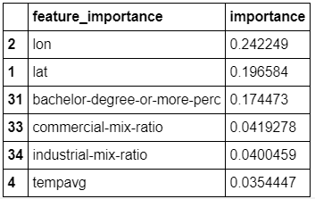
Very interesting to see that our “bachelor-degree-or-more-percentage” and “commercial/industrial-mix-ratio” features to be among the top predictors of crime for this model.

Overfitting

In an effort to better understand the point at which our model would overfit our data, we’ve created an overfit tree model called “overfit_cv_tree” with the following parameters:

overfit_cv_tree = DecisionTreeClassifier(max_depth=30)

overfit_cv_tree model produced a training accuracy of .8878 and a test accuracy of .29082. We’ve noticed that depths of 20 and greater are most likely overfitting given the large difference in train and test accuracy. We’ve utilized a depth of 30 to ensure overfitting.

Bagging

In an effort to further reduce the variance of our decision tree we created a bagging model using 55 trees. We then fit our new bagging model, titled “bagging_model” to 5,000 random samples. Each tree produced a training accuracy of .0487 and a test accuracy of .0472.

Bootstraps Affects & Bagging Ensemble’s Performance

To better understand how the number of bootstraps affects our bagging ensemble’s performance we’ve plotted model accuracy scores across several bootstrapepd models below:

bootstrap_accuracy

The baselines of course are flat because they are only run once. The bagging model for the first couple runs starts off at a higher accuracy only to decrease and level off. This illustrates the need to aggregate all of our bootstrapped models for a combined prediction.

Random Forest

Continuing with our goal to reduce model variance and average multiple deep decision trees we want to pass similar parameters to a random forest model. After thorough testing of model accuracy our final random forest model titled “random_forest” was created with the following parameters:

random_forest = RandomForestClassifier(n_estimators=55, max_depth=13, max_features='sqrt')

Random forest randomly selects a subset of predictors to split on. Therefore the first split can vary based on what subset of predictors is being used. Bagging does not subset the predictors so is always using the same best predictor. Random forest can possibly capture more variance in the data because it is aggregating trees that are more varied. Theoretically random forest should therefore be able to get higher accuracies than bagging.

Our random_forest model produced a training accuracy of .4243 and a test accuracy of .3501

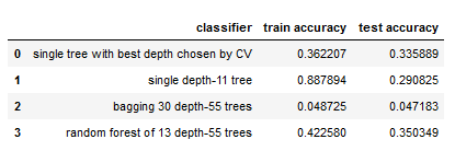
Accuracy Comparison:

The table below shows the train and test accuracy across the decision tree models we’ve built. Worth noting that our random forest is our highest performing model at this time.

Boosting

We’ll now utilize boosting, another type of ensemble method, where each new model is trained on a dataset weighted towards observations that the current set of models predicts incorrectly. We’ll use AdaBoost (ada), or Adaptive Boosting, to transform our weaker classifiers into stronger ones.

After initial testing, our best performing ada model is defined with the following parameters:

ada = AdaBoostClassifier(DecisionTreeClassifier(max_depth=6), n_estimators=200, learning_rate=0.05)

The plot below illustrates the accuracy scores by iteration number of our best performing ada model.

In an effort to demonstrate that we’ve chosen the optimal ada model we’ve also plotted the results of model depths of 5-8 for comparison purposes:

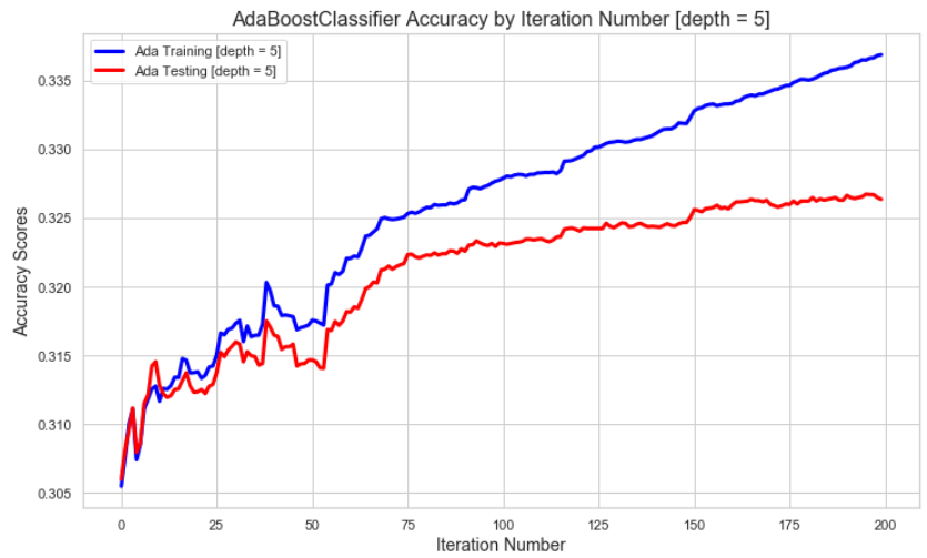
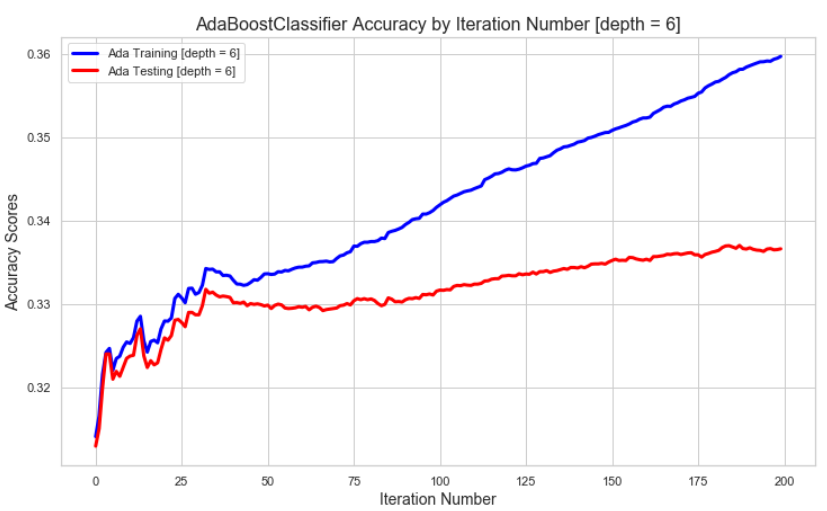
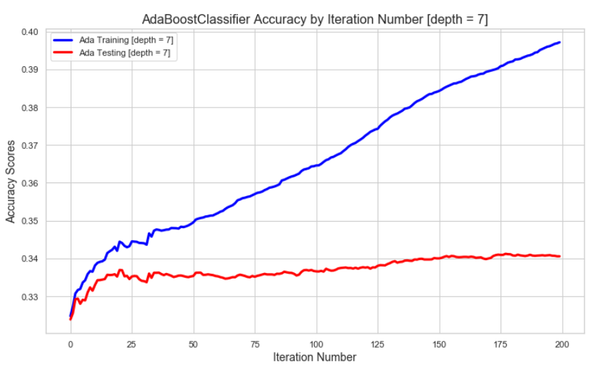
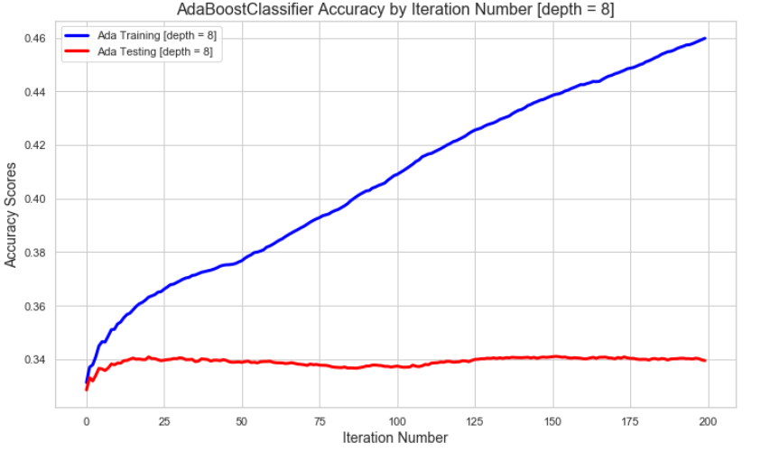
ada_boost_5 ada_boost_6 ada_boost_7 ada_boost_8

The lower tree depths require more boosting iterations to reach the best accuracies that are not overfit. Though, in this case the max accuracies are similar at depth=5 does have a lower max accuracy even after 200 iterations (with data where the first predictor is only marginally better this will be more pronounced). The higher the tree depth the lower the number of iterations where boosting starts to overfit.

The training accuracy mostly remains between 0.30-0.46 (test accuracy ranges between 0.31-0.34) but as the depth increases the max training accuracy gets closer and closer to 1.0. At higher depths, boosting is greatly overfitting the training data.

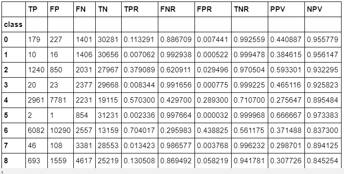
Best Model: Random Forest Results

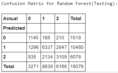
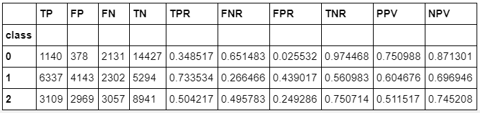
Random Forest appears to have outperformed all other models and warrants further discovery. Below we’ve added confusion matrices to illustrate our predictions vs. actual values by crime class. We’ve also added true positive, false positive, false negative, true negatives, their rates and predictive values by class. Confusion matrices

confusion_matrix_rf

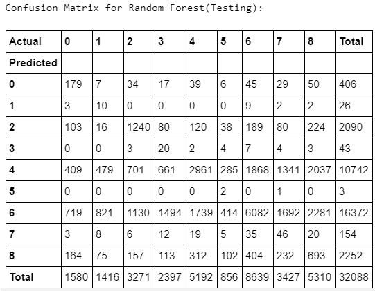
Key for matrix below: {[TP = True Positive], [FP = False Positive], [FN = False Negative], [TN = True Negative], [TPR = True Positive Rate], [FNR = False Negative Rate], [FPR = False Positive Rate], [TNR = True Negative Rate], [PPV = Positive Predictive Value], [NPV = Negative Predictive Value]}

confusion_matrix_rf_2

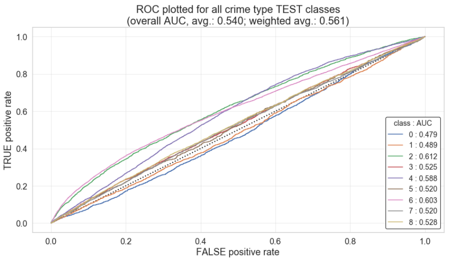
AUC

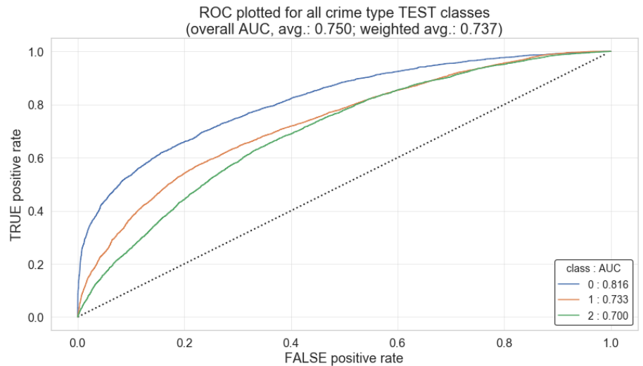
Finally, to see how well our best model performs we examine the area under the curve. Our Random Forest AUC Average came to 0.5406 and our Random Forest Weighted AUC Average came to 0.5569. The plot below illustrates our random forest model performance across crime class:

roc_auc

Different Subsets of the Data

The Decision Tree subset data notebook can be found here.

We are using the full crime dataset along with customized categories that we created. How the data is subset and how the categories are chosen can greatly impact the accuracy our models achieve. Our framework is extensible enough to accommodate for different subsets and categories based on requirements.

For example below are the results for a random forest run on a subset of the data with three classes: (drugs-substances, theft, violence-aggression)

Much better model scores:
Accuracy 0.3503 –> 0.5856, AUC 0.5406 –> 0.7495, Weighted AUC 0.5569 –> 0.7367

Testing Accuracy = 0.5856

AUC Average = 0.7495

Weighted AUC Average = 0.7367

confusion_matrix_rf_subset

confusion_matrix_rf_2_subset

roc_auc_subset